As indicated by the name, the predictive rating is the best of my ratings in its predictive power. From these ratings, you can determine two things. One is the odds of a team winning a game against an opponent; the other is the expected final score. The obvious disclaimer applies to this -- although I have done the best possible, there is no guarantee as to the accuracy of predictions. Specifically, these ratings do not account for injuries to key players, nor do they account for specific matchups in the games. A form at the bottom of the rankings page will call a CGI script that will do the calculations below; the information here is just for reference. (For interest, there is also a CGI script that will show a plot of the game-by-game team strength as a function of time during the season.)
The odds of a team winning is calculated as:
score = CP ( rating - opponent +/- home field ), score = CP [ ( rating - opponent +/- home field ) / sqrt ( 1 + 1/ngames1 + 1/ngames2 ) ],| x | CP(-x) | CP(x) |
|---|---|---|
| 0.0 | 0.500 | 0.500 |
| 0.5 | 0.309 | 0.691 |
| 1.0 | 0.159 | 0.841 |
| 1.5 | 0.067 | 0.933 |
| 2.0 | 0.023 | 0.977 |
Example: A rematch of the 2002 NCAA hockey championship game, Maine at Minnesota. From the 2002 hockey ratings, Minnesota's predictive rating is 1.177 and Maine's is 0.993, while the home field factor is 0.205. This gives Minnesota a 0.389 point edge. Calculating CP(0.389), one finds a 65.1% chance of Minnesota winning a rematch. Had the game been played at Maine, the odds would have been nearly 50-50, emphasizing the importance of neutral venues for championship games. (Using the 'predict score' form on the web site gives 64.8%, the difference resulting from rounding.)
A calculation that is more complex is the prediction of game outcomes, which is done using the factor inside CP above as well as the team's scoring ratings, SCORING. The SCORING rating is an indication of whether the team tends to be involved in high- or low-scoring games.
To determine the most likely score, use:
   x = ( rating - opponent +/- home field ) * F
   s = exp ( SCORING1 + SCORING2 )
   y = [ x^2 + sqrt ( x^4 + 16 * s) ] /2
   score = scale * [ y + x*sqrt(y) ] /2
   margin = scale * x * sqrt(y)
total = scale * y,Example: A rematch of the 2002 men's college basketball championship game, Indiana vs. Maryland. First we calculate x from the ratings (1.869 for Maryland and 1.600 for Indiana), and ignoring the home court factor of 0.405 since the game was at a neutral site. This gives x=0.269 for Maryland. (In this example, M is omitted.)
Second, we calculate s using the teams' scoring ratings (3.657 for Maryland, 3.385 for Indiana). This gives s=1144, and consequently y=67.67.
Finally, we determine the expected scores, which are 75.1 for Maryland and 70.4 for Indiana. The actual score was much lower (64-52 Maryland), since Indiana was able to slow the tempo of the game more than expected and more than they would have likely been able to do in a rematch. (The score predicting program makes a slightly more accurate calculation than this.)
In terms of ranking offenses and defenses, two similar ratings are shown that indicate the quality of opponent that would produce an average score against the team. Solving the above equations for the case where an opponent's SCORING is set to the league average, one finds:
   OFFENSE = rating + (exp(SCORING)-exp(average)) / sqrt(exp(SCORING)+exp(average))
DEFENSE = rating - (exp(SCORING)-exp(average)) / sqrt(exp(SCORING)+exp(average)),There is a form at the bottom of the ratings pages that can be used to make these calculations based on the current predictive ratings. Since this is intended for educational purposes rather than gambling purposes, I have intentionally omitted a calculation of the odds of a specific point spread or over/under being met.
Because of significant differences between ballparks, baseball ratings include an adjustment, in the BALLPARK column, which is applied to all games played at the team's home ballpark. This is added to SCORING1 and SCORING2 in the above equation. This factor is not used in the web prediction scripts at present, which means that baseball score predictions are not as accurate as those in other sports (though odds of winning are calculated correctly). In sports other than baseball, BALLPARK is set equal to zero. To adjust the predictions for the home field factor, multiply all scores (each team's predicted score, the predicted difference, and the predicted total) by exp(BALLPARK/2). For example, Colorado's BALLPARK value from 2004 is 0.597, indicating that all scores predicted in that ballpark should be multiplied by 1.35.
Finally, note that the ratings used by the prediction form on this website incorporate preseason predictions, even after teams have played sufficient games that the published ratings do not use the preseason prediction. Analysis of historical data shows that this provides more accurate predictions, as even a full season's worth of NFL games leaves an uncertainty of 0.25 (one-sigma) in the predictive rating.
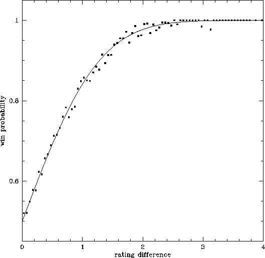
Given the large number of games played during the time I have been doing ratings, a valid question is how well the predictions have fared in the past. To answer this, I have retroactively calculated the odds of winning each game, with team ratings recalculated ignoring the game in question. The result is showm blow. The dots indicate the observed win probabilities of all games, while the curve indicates the Gaussian error function. Clearly the ratings work quite well, and more significantly the Gaussian error function is a good approximation of the probabilities.

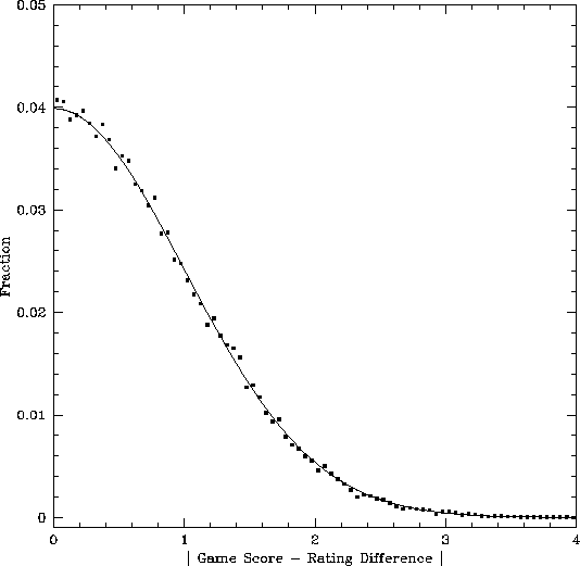
A second test can be done to compare the score predictions of the games. The plot below shows the distribution of game score (G) minus rating difference (dr) values. As above, the curve is the expected distribution if randomness is Gaussian. Once again, the results are in excellent agreement with the predictions. What may surprise some people is that the distribution is virtually identical considering; "common wisdom" would indicate that results from mismatches are more random than those from evenly-matched opponents.

Note: if you use any of the facts, equations, or mathematical principles on this page, you must give me credit.